Original date published: October 7, 2024
Exploring NVIDIA Newton - Advanced GPU-Accelerated Physics Simulation
An introductory guide to NVIDIA Newton's capabilities for creating realistic physics simulations with GPU acceleration and differential programming
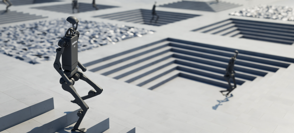
Unitree H1 Humanoid robot in Nvidia GPU accelerated simulation
As the capabilities of physical AI systems accelerate, engineers and developers need more accurate physics simulation environments that reduce the sim-to-real gap. Simulation can be used to scale robot learning systems to use the collective learning of multiple robot instances over an accelerated period of time. Traditional CPU-based physics simulators such as the original MuJoCo implementation struggle to render complex environment dynamics in simulation. Physics simulation can leverage the parallelization capabilities provided by GPUs to enable powerful and realistic physics simulation using tools like NVIDIA Newton.
NVIDIA Newton is written using the NVIDIA Warp library which allows for writing differential spatial computing kernels in Python. Newton extends and generalizes Warp's simulation module and integrates MuJoCo Warp as its primary backend. Newton emphasizes GPU computation and supports the open Universal Scene Description (OpenUSD) library.
Building Simulation Examples with NVIDIA Newton
To start, we will look at a simple pendulum simulation provided in the Newton repository. The pendulum has two joints and swings freely in the air, demonstrating the core physics simulation capabilities.
Two-Link Pendulum Implementation
import warp as wp
import newton
import newton.examples

class PendulumSimulator:
    def __init__(self, viewer):
        # setup simulation parameters first
        self.fps = 100
        self.frame_dt = 1.0 / self.fps
        self.sim_time = 0.0
        self.sim_substeps = 10
        self.sim_dt = self.frame_dt / self.sim_substeps

        # we'll store a reference to the viewer in the simulator class
        self.viewer = viewer

        # we'll define a model body builder object
        builder = newton.ModelBuilder()

        # add the pendulum articulation to the model
        builder.add_articulation(key="2-link-pendulum")

        # define the size of the links
        hx = 1.0
        hy = 0.1
        hz = 0.1

        # create first link
        link_0 = builder.add_body()
        builder.add_shape_box(link_0, hx=hx, hy=hy, hz=hz)
        # create second link
        link_1 = builder.add_body()
        builder.add_shape_box(link_1, hx=hx, hy=hy, hz=hz)

        # add joints
        rot = wp.quat_from_axis_angle(wp.vec3(0.0, 0.0, 1.0), -wp.pi * 0.5)
        # add the first joint
        builder.add_joint_revolute(
            parent=-1,
            child=link_0,
            axis=wp.vec3(0.0, 1.0, 0.0),
            # rotate pendulum around the z-axis to appear sideways to the viewer
            parent_xform=wp.transform(p=wp.vec3(0.0, 0.0, 5.0), q=rot),
            child_xform=wp.transform(p=wp.vec3(-hx, 0.0, 0.0), q=wp.quat_identity()),
        )
        # add the second joint
        builder.add_joint_revolute(
            parent=link_0,
            child=link_1,
            axis=wp.vec3(0.0, 1.0, 0.0),
            parent_xform=wp.transform(p=wp.vec3(hx, 0.0, 0.0), q=wp.quat_identity()),
            child_xform=wp.transform(p=wp.vec3(-hx, 0.0, 0.0), q=wp.quat_identity()),
        )

        # add ground plane
        builder.add_ground_plane()

        # finalize model
        self.model = builder.finalize()

        # implement the physics solver
        self.solver = newton.solvers.SolverXPBD(self.model)

        # initialize the state variables
        self.state_0 = self.model.state()
        self.state_1 = self.model.state()
        self.control = self.model.control()
        self.contacts = self.model.collide(self.state_0)

        self.viewer.set_model(self.model)

        # not required for MuJoCo, but required for other solvers
        newton.eval_fk(self.model, self.model.joint_q, self.model.joint_qd, self.state_0)

        self.capture()
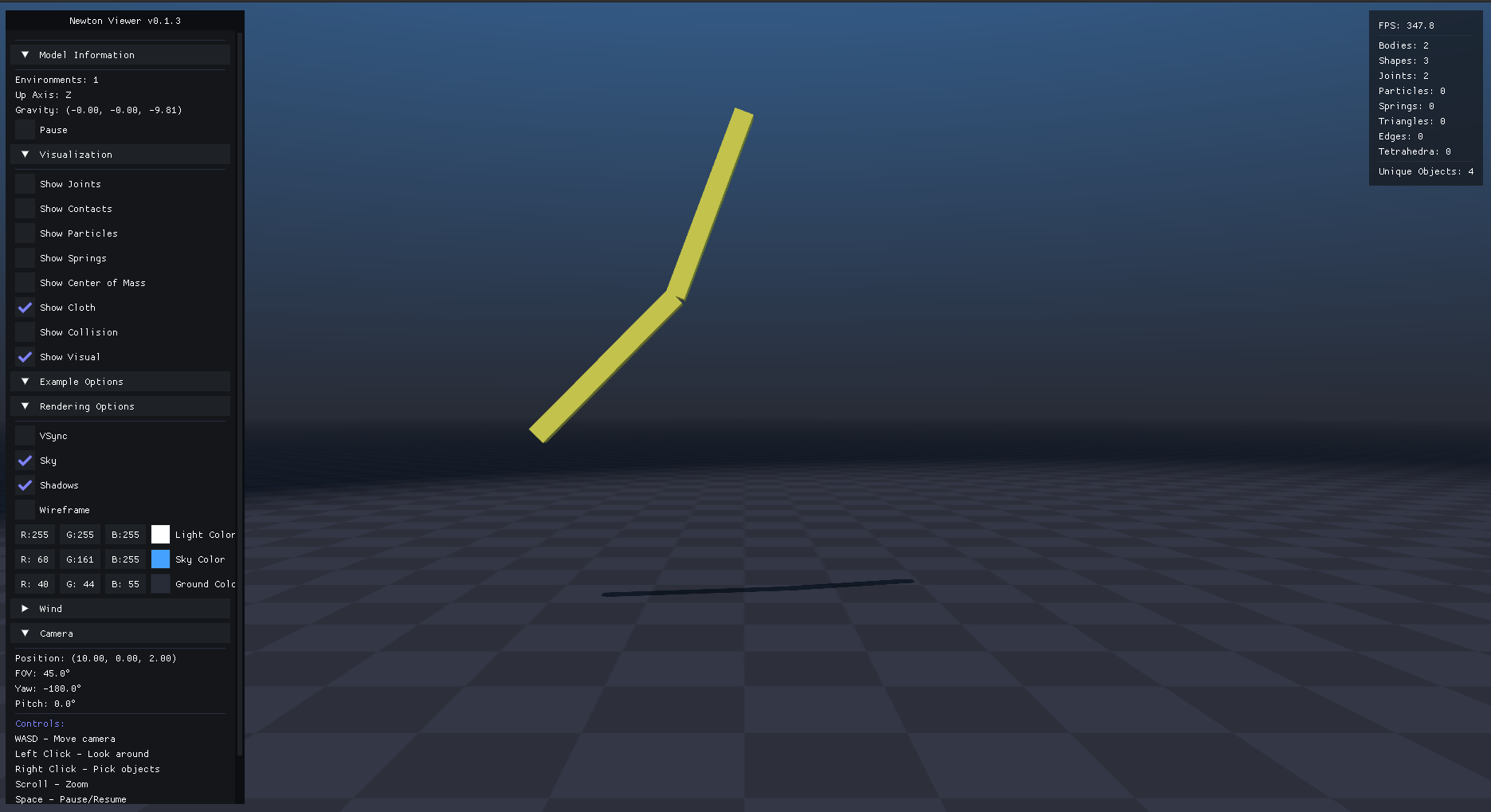
Two-Link Pendulum in NVIDIA Newton Viewer showing the simulation environment
We can now observe how the model works in the simulated environment using the graphical window shown above. We can adjust parameters like wind to see how changing the physical parameters affects the model behavior.
Extending to Three Links
We can now extend the basic 2-link pendulum into a 3-link pendulum and see how the simulation model changes accordingly.
class ThreeLinkPendulumSimulator:
    def __init__(self, viewer):
        # setup simulation parameters first
        self.fps = 100
        self.frame_dt = 1.0 / self.fps
        self.sim_time = 0.0
        self.sim_substeps = 10
        self.sim_dt = self.frame_dt / self.sim_substeps

        self.viewer = viewer

        builder = newton.ModelBuilder()
        builder.add_articulation(key="pendulum")

        hx = 0.7
        hy = 0.1
        hz = 0.1

        # create three links
        link_0 = builder.add_body()
        builder.add_shape_box(link_0, hx=hx, hy=hy, hz=hz)

        link_1 = builder.add_body()
        builder.add_shape_box(link_1, hx=hx, hy=hy, hz=hz)

        link_2 = builder.add_body()
        builder.add_shape_box(link_2, hx=hx, hy=hy, hz=hz)

        # add joints
        rot = wp.quat_from_axis_angle(wp.vec3(0.0, 0.0, 1.0), -wp.pi * 0.5)
        builder.add_joint_revolute(
            parent=-1,
            child=link_0,
            axis=wp.vec3(0.0, 1.0, 0.0),
            # rotate pendulum around the z-axis to appear sideways to the viewer
            parent_xform=wp.transform(p=wp.vec3(0.0, 0.0, 5.0), q=rot),
            child_xform=wp.transform(p=wp.vec3(-hx, 0.0, 0.0), q=wp.quat_identity()),
        )
        builder.add_joint_revolute(
            parent=link_0,
            child=link_1,
            axis=wp.vec3(0.0, 1.0, 0.0),
            parent_xform=wp.transform(p=wp.vec3(hx, 0.0, 0.0), q=wp.quat_identity()),
            child_xform=wp.transform(p=wp.vec3(-hx, 0.0, 0.0), q=wp.quat_identity()),
        )

        # add the third joint
        builder.add_joint_revolute(
            parent=link_1,
            child=link_2,
            axis=wp.vec3(0.0, 1.0, 0.0),
            parent_xform=wp.transform(p=wp.vec3(hx, 0.0, 0.0), q=wp.quat_identity()),
            child_xform=wp.transform(p=wp.vec3(-hx, 0.0, 0.0), q=wp.quat_identity()),
        )

        # add ground plane
        builder.add_ground_plane()

        # finalize model
        self.model = builder.finalize()
        self.solver = newton.solvers.SolverXPBD(self.model)

        # Initialize state variables and contacts
        self.state_0 = self.model.state()
        self.state_1 = self.model.state()
        self.control = self.model.control()
        self.contacts = self.model.collide(self.state_0)

        self.viewer.set_model(self.model)
        newton.eval_fk(self.model, self.model.joint_q, self.model.joint_qd, self.state_0)
        self.capture()
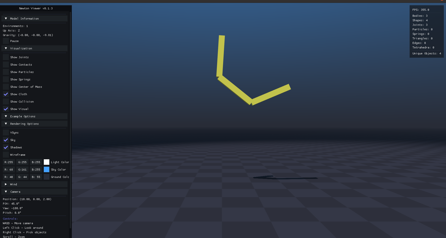
Three-Link Pendulum showing increased complexity and more dynamic behavior
Key Features and Benefits
GPU Acceleration
NVIDIA Newton leverages GPU parallelization to handle complex physics calculations that would be computationally expensive on traditional CPU-based simulators. This enables:
- Faster simulation times: Multiple physics calculations can be performed in parallel
- Higher fidelity simulations: More complex environmental dynamics can be modeled
- Scalable robot learning: Multiple robot instances can learn simultaneously
Integration with NVIDIA Warp
Newton's foundation on NVIDIA Warp provides:
- Differential programming: Enables gradient-based optimization of physical systems using automatic differentiation
- Python-native development: Write physics kernels directly in Python with CUDA compilation
- Spatial computing: Advanced mathematical operations for 3D transformations and physics based on Warp's spatial math library
OpenUSD Support
The integration with Universal Scene Description (OpenUSD) offers:
- Industry-standard asset pipeline: Seamless integration with existing 3D workflows and USD ecosystem
- Cross-platform compatibility: Works with various 3D software and rendering engines like Blender, Maya, and Houdini
- Collaborative development: Teams can work with standardized scene descriptions and version control
Applications in Robotics and AI
NVIDIA Newton provides a new way to model complex physical objects and mirror accurate real-world physical dynamics. This capability is particularly valuable for:
- Reinforcement learning: Training robots in simulation before real-world deployment, following approaches like PPO and SAC
- Sim-to-real transfer: Reducing the gap between simulated and real-world performance using techniques like domain randomization
- Multi-agent systems: Simulating interactions between multiple robotic agents in complex environments
- Physical AI development: Creating intelligent systems that understand and interact with the physical world, advancing the field of embodied AI
Conclusion
NVIDIA Newton represents a significant advancement in physics simulation technology, combining the power of GPU acceleration with the flexibility of Python development. By providing accurate, high-performance physics simulation capabilities, Newton enables researchers and developers to create more sophisticated AI systems that can effectively bridge the gap between simulation and reality.
The pendulum examples demonstrate how easily developers can create complex articulated systems and observe realistic physical behavior. As the field of physical AI continues to evolve, tools like NVIDIA Newton will play a crucial role in enabling the next generation of intelligent robotic systems.
Last updated at: October 7, 2024